Understanding Variational Auto-Encoders (VAE)

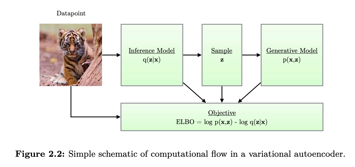
Disclaimer: this post is heavily based on Introduction to variational auto-encoders, Kingma & Welling, 2019[^intro-vae]

Introduction

As of April 2024, the VAE Paper from 2013 has been cited more than 34 thousand times. What can we learn from the variational auto-encoder ?

The framework of VAE provides a principled method for jointly learning deep latent-variable models and corresponding inference models using stochastic gradient descent.

It has a wide array of application: - generative modelling - semi-supervised learning - representation learning

The VAE can be viewed as two coupled, but independently parameterized models: - the encoder or recognition model - the decoder or generative model

The recognition model is the approximate inverse of the generative model according to Bayes rule.

The idea of training an inference network to “invert” a generative network, rather than running an optimization algorithm to infer the latent code, is called amortized inference.

VAE vs vanilla AE

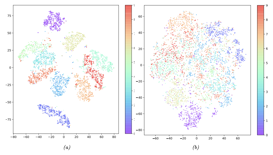
The main advantage of a VAE over a deterministic autoencoder is that it defines a proper generative model that can create sensible-looking novel images by decoding prior samples z \sim \mathcal{N}(0, I). By contrast, an autoencoder only knows how to decode latent codes derived from the training set, so does poorly when fed random inputs.

The reason behind this is that the VAE embeds images into Gaussians in latent space, whereas the AE embeds images into points, which are like delta functions. The advantage of using a latent distribution is that it encourages local smoothness since a given image may map to multiple nearby places, depending on the stochastic sampling. By contrast, in an AE the latent space is not smooth, so images from different classes often en up next to each other.

tSNE projection of a 20-dimensional latent space for MNIST with (a) VAE (b) deterministic AE

Key ideas

3 key ideas according to Bishop [^deep-bishop]:

• Evidence Lower Bound (ELBO) to approximate likelihood function (leads to a close relationship to EM algorithm)
• Amortized inference in which a second model, the encoder network, is used to approximate the posterior distribution over latent variables in the E step, rather than evaluating the posterior distribution for each data point exactly
• Making the training of the encoder model tractable using the reparameterization trick

Concept

Inference model / recognition model / encoder: q_{\mathbf{\phi}} (\mathbf{z}|\mathbf{x}) where \phi are the variational parameters.

We optimize these parameters such that:

q_{\mathbf{\phi}} (\mathbf{z}|\mathbf{x}) \approx p_{\mathbf{\theta}}(\mathbf{z}|\mathbf{x})

the distribution q_{\mathbf{\phi}} (\mathbf{z}|\mathbf{x}) can be parameterized using deep neural networks. In this case, the variational parameters \phi include the weights and biases of the neural network. For example:

(\mathbf{\mu}, \log \mathbf{\sigma}) = \mathrm{EncoderNeuralNet}_{\phi}(\mathbf{x})

q_{\mathbf{\phi}} (\mathbf{z} | \mathbf{x}) = \mathcal{N}(\mathbf{z}; \mathbf{\mu}, \mathrm{diag}(\sigma))

The VAE learns stochastic mappings between observed x-space, whose empirical distribution is complicated, and a latent z-space whose distribution is simple (here spherical)

Evidence Lower Bound (ELBO)

Evidence lower bound / Variational lower bound.

We define the \mathrm{ELBO} as:

\mathcal{L_{\theta,\phi}}(\mathbf{x}) = \mathbb{E_{q_{\phi}(\mathbf{z}|\mathbf{x})}}[\log p_{\theta}(\mathbf{x}, \mathbf{z}) - \log q_{\phi}(\mathbf{z} | \mathbf{x})]

It’s possible to prove the following key equation:

\log p_{\theta}(\mathbf{x}) = \mathcal{L_{\theta,\phi}}(\mathbf{x}) + D_{KL}(q_{\mathbf{\phi}} (\mathbf{z} | \mathbf{x}) || p_{\mathbf{\theta}} (\mathbf{z} | \mathbf{x}))

The point is that the KL-divergence is always non-negative, so the ELBO is a lower bound on the log-likelihood of the data (marginal log-likelihood).

Two for One

Maximizing the ELBO will have two effects: - maximize the marginal likelihood p_{\theta}(x) => the generative model will become better - It will minimize the KL divergence of the approximation q_{\mathbf{\phi}} (\mathbf{z} | \mathbf{x}) from the true posterior p_{\theta} (\mathbf{z} | \mathbf{x}), so the approximation becomes better.

Simple schematic of computational flow in a variational autoencoder.

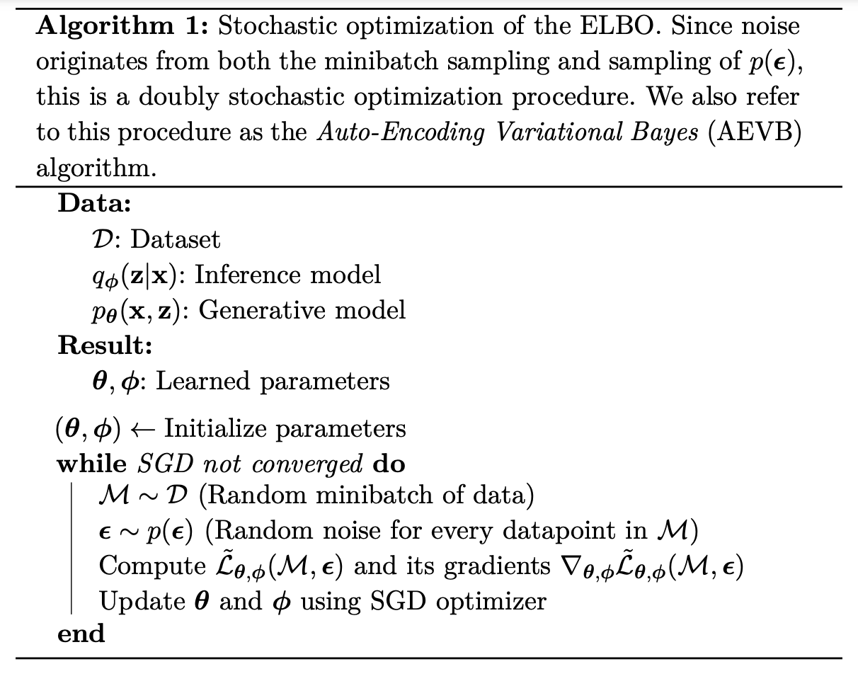
Stochastic gradient-based optimization of the ELBO

The individual-datapoint ELBO, and its gradient is, in general, intractable. However, good unbiased estimators exist, as we will show, such that we can still perform minibatch SGD:

• Unbiased gradients of the ELBO with respect to (w.r.t.) the generative model parameters \theta are simple to obtain, with a Monte Carlo estimator.
• However, unbiased gradients w.r.t. the variational paramters \phi are more difficult to obtain because the expectation is taken w.r.t. to a function of \phi.

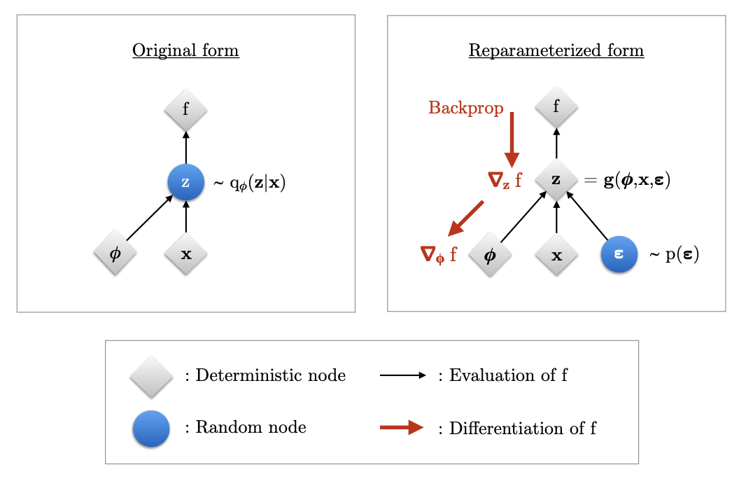
For continuous latent variables, we can use a reparameterization trick to compute unbiased estimates of the double gradient.

Reparameterization Trick

We express the random variable z \sim q_{\mathbf{\phi}} (\mathbf{z} | \mathbf{x}) as some differentiable and invertible transformation of another r.v. \epsilon, given x and \phi:

z = g(\epsilon, \phi, \mathbf{x})

\epsilon \sim p(\epsilon) is a noise sample.

Reparameterization trick to backpropagate gradients

With the reparam trick, we can rewrite the ELBO as:

\mathcal{L_{\theta,\phi}}(\mathbf{x}) = \mathbb{E_{p(\epsilon)}}[\log p_{\theta}(\mathbf{x}, \mathbf{z}) - \log q_{\phi}(\mathbf{z} | \mathbf{x})]

where z = g(\epsilon, \phi, \mathbf{x}).

We can then form a simple Monte-Carlo estimator \tilde{\mathcal{L_{\theta, \phi}}}(x) of the individual-datapoint ELBO where we use a single noise sample \epsilon from p(\epsilon):

\epsilon \sim p(\epsilon) z = g(\phi, x, \epsilon) \tilde{\mathcal{L_{\theta, \phi}}}(x) = \log p_{\theta}(x, z) - \log q_{\phi}(z|x)

The two terms above correspond to the generative model (decoder) and the recognition model (encoder).

The VAE algorithm - stochastic optimization of the ELBO

Computing \log q_{\phi}(z|x)

Computation of the estimator of the ELBO requires computation of the density $ q_{}(z|x)$, given a value of x and given a value of z or equivalently \epsilon.

This log-density is a simple computation, as long as we choose the right transformation g.

As long as g(.) is an invertible function, the densities of \epsilon and z are related as:

\log q_{\phi} (z|x) = \log p(\epsilon) - \log d_{\phi}(x, \epsilon)

Where the second term is the log of the absolute value of the determinant of the jacobian matrix \partial z \over \partial \epsilon.

This is the log-determinant of the transformation from \epsilon to z.

We will see that we can build very flexible transformations g(.) for which the log-determinant is simple to compute, resulting in highly flexible inference models q_{\phi}(z|x).

Factorized Gaussian posteriors

(\mathbf{\mu}, \log \mathbf{\sigma}) = \mathrm{EncoderNeuralNet}_{\phi}(\mathbf{x})

q_{\mathbf{\phi}} (\mathbf{z} | \mathbf{x}) = \prod_i q_{\phi}(z_i | \mathbf{x}) = \prod_i \mathcal{N}(z_i; \mu_i, \sigma_i^2)

After reparameterization, we can write instead:

\epsilon \sim \mathcal{N}(0, \mathbf{I})

(\mathbf{\mu}, \log \mathbf{\sigma}) = \mathrm{EncoderNeuralNet}_{\phi}(\mathbf{x})

z = \mu + \sigma \odot \epsilon

The jacobian of the transformation from \epsilon to z is:

{\partial z \over \partial \epsilon} = \mathrm{diag}(\sigma)

Thus the log-determinant is

\log d_{\phi}(x, \epsilon) = \sum_i \log \sigma_i

And the posterior density when z = g(\epsilon, \phi, x) is:

\log q_{\phi} (z|x) = \sum_i \log \mathcal{N}(\epsilon_i; 0, 1) - \log \sigma_i

Estimation of the Marginal Likelihood

After training a VAE, we can estimate the probability of data under the model using importance sampling.

Since the marginal likelihood of a datapoint is:

\log p_{\theta}(x) = \log \mathbb{E_{q_{\phi}(z|x)}}[{p_{\theta}(x, z) \over q_{\phi}(z|x)}]

Taking random samples z^{(l)} \sim q_{\phi}(z|x), a Monte-Carlo estimator of this is:

\log p_{\theta}(x) \approx \log {1 \over L} \sum_{l=1}^L {p_{\theta} (x, z^{(l)}) \over q_{\phi}(z^{(l)}|x)}

With a large L, the approximation becomes a better estimate of the marginal likelihood.

Follow-up work

Here are some important applications for deep generative models and VAE:

• Representation learning
  • data-efficient learning, such as semi-supervised learning
  • visualisation of data as low-dimensional manifolds
• Artificial creativity: plausible interpolation between data and extrapolation from data

Representation learning

For supervised learning tasks, we want to learn a conditional distribution.: to predict the distribution over the possible values of a variable given the value of some other variable. One example is image classification. For this task, deep neural nets such as CNNs are very good with large amounts of data.

However, when the number of labaled examples is low, solutions with purely supervised approaches exhibit poor generalization to new data. In this case, generative models can be used as an effective type of regularization. One strategy is to optimize the classification model jointly with a VAE over the input variables, sharing parameters between the two. This procedure improves the data efficiency of the classification solution.

Example: < 1% classification error on MNIST when trained with only 10 labeled images per class, i.e. 99.8% of the labels in the training set removed. Some works even show that VAE-based semi-supervised learning can even do well when only a single sample per class is presented.

Understanding of data and artificial creativity

• Chemical design: learn a continuous representation (laten space) of discrete structures of molecules to do gradient-based optimization towards certain properties.

Chemical design - gradient-based optimization on latent space

• Natural language synthesis: interpolate between sentences, imputation of missing words.
• Image (re-)synthesis: modification of an image in latent space along a smile vector

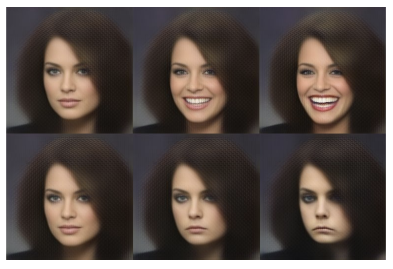Modifications of an image along a smile vector

Conclusion

Parameterizing the conditional distributions of directed probabilistic models with differentiable deep neural networks can make them very flexible.

The main contribution of VAEs is a framework for efficient and scalable gradient-based variational posterior inference and approximate maximum likelihood learning.

References

[^intro-vae] An Introduction to Variational Autoencoders, Kingma & Welling (original VAE authors), 2019

[^deep-bishop] Deep Learning - Foundations and concepts, Bishop & Bishop, 2023, chapter 19.2 page 569 (slider 581)

Probabilistic Machine Learning: An introduction, Kevin P. Murphy, 2022

Probabilistic Machine Learning: Advanced Topics, Kevin P. Murphy, 2023

Sebastian Callh’s blog post