I first learned about bayesian statistics in a job posting for an internship. At the time, I was about 20 years old and had never heard of it. The concept was so alien to me that I first read bayesian interference. I figured it had something to do with optics, such as the Michelson interferometer that I (still) fear.
Fast-forward a small decade and I now consider myself a (secular) bayesian. What is bayesian statistics really about ?
Bayes’ theorem
In the beginning of every probability book, you will see Bayes’ thoerem for events proudly stated as a direct consequence of the definition of conditional probability and the product (chain) rule. I argue here that it is not really helpful to think of bayes this way. If you wonder what Bayes’ theorem is, you can look it up online.
A biased coin
When I was in high school, I remember that we saw in a book that if you toss a coin 3 times and it leads 3 heads, the probability that the next toss will lead head too is … 0.5 (50%). I was a bit surprised by the result, because I overlooked the crucial fact that we knew the coin was unbiased, i.e. that it always leads to heads with a probability of 0.5.
However, if you don’t know if the coin is biased or not, then your belief that the next coin toss is going to lead heads should surely be a little higher than tails. A relevant question you can ask yourself is: at what odds would you accept to bet on tails ? Assuming you want your expected gain to be positive of course.
The reverend Thomas Bayes
Born c. 1701, Thomas Bayes was a pioneer of statistics, and a minister of the Church. Coincidentally, these days some people are so deep into the Bayesian doctrine that we can consider them as being part of the Bayesian church.
In 1763 was published An Essay towards solving a Problem in the Doctrine of Chances, 2 years after Bayes’ death. In it, he states in the beginning the Bayes’ theorem as we know it. On wikipedia we can read:
it does not appear that Bayes emphasized or focused on this finding. Rather, he focused on the finding the solution to a much broader inferential problem:
“Given the number of times in which an unknown event has happened and failed [… Find] the chance that the probability of its happening in a single trial lies somewhere between any two degrees of probability that can be named.”
Sounds like he was wondering about the coin toss problem !
Inverse probability
During the 18 & 19th century, mathematicians such as Laplace and De Morgan refer to the inverse probability for the probability distribution of an unobserved variable. The term Bayesian was coined by Ronald Fisher in 1950, with the development of frequentism, to refer to the same thing.
Intuitively, statistics is about inverse problems : if you have some unobserved variables and possibly observed variables (often in the form of events), how can you assess the distribution of the unobserved variable ?
The inference theorem
In Bayesian inference, parameters are random and data is not.
Here is the formula that we care about in inferential bayesian statistics:
\mathrm{posterior} \propto \mathrm{prior} \times \mathrm{likelihood}
The \propto sign means proportional to, as such a \propto b means a = C \times b for some constant C.
In more precise terms, let \theta be the unobserved random variable that we care about (weights & biases in machine learning for instance).
Let p(\theta) denote the distribution of \theta. More rigorously, p in this post loosely denotes either the probability of an event or the probability density (or probability mass function) of a random variable. When I write distribution it often means density of the random variable.
Let D (for Data) denote our observed data, for instance D = (\mathbf{x}, \mathbf{y}) = (x_i, y_i)_i for a regression or classification problem. Then the above formula can be written more precisely:
p(\theta | D) \propto p(\theta) \times p(D | \theta)
The prior distribution p(\theta) is the probability distribution of the unobserved random variable (r.v.) of interest a priori, i.e. without having seen any data / observed related r.v. / events. It may reflect your knowledge about the world.
The likelihood p(D | \theta) is the probability of the data conditioned on this unobserved random variable. This may sounds paradoxical: how can we condition on something we don’t observe ? Well, remember that this is a function of the unobserved random variable. As such, the likelihood is NOT a density, it doesn’t integrate to 1. We can put it another way: If we knew the unobserved variable, how likely would the data (events) we have observed be ?
The posterior distribution p(\theta | D) is what we ultimately care about. It describes the distribution of the unobserved r.v. \theta condtioning on the data that we’ve collected, i.e. events that happened.
What to make of this formula ?
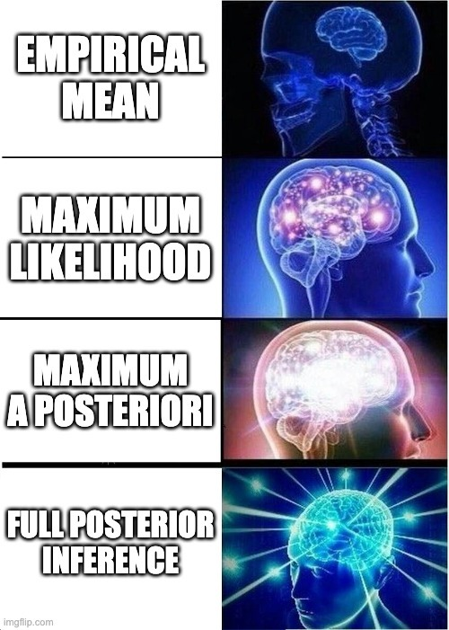
There are mainly 3 types of inference methods that we can leverage based on the above formula:
- Maximum likelihood estimation (MLE): we seek one point estimate of \theta based on observations and the likelihood
- Maximum a posteriori (MAP): we seek one point estimate of \theta based on observations and prior knowledge - likelihood and prior
- Full posterior inference: we seek representative samples from the posterior distribution of \theta based on the inference formula.
Maximum Likelihood
In this setting, we just optimize the likelihood to get the argmax. In this case, we ignore the prior and the posterior ; hence, we don’t really use the inference formula. Kevin Murphy refers to MLE and MAP as poor man’s Bayes.
This method is convenient because we can just optimize the function, with e.g. the gradient, and find the value of \theta that maximizes the likelihood function. We can either compute the gradient in closed form and see where it vanishes, or run an iterative algorithm such as (stochastic) gradient descent.
In practice, we dont maximize the likelihood function but rather we minimize the negative log-likelihood function (NLL) with the logarithm function:
NLL(\theta) := - \log p(D | \theta)
Note that in the case of a gaussian likelihood, for a regression, the negative log-likelihood is then equal (up to a constant) to the mean-squared error loss function, widely used in machine learning. In the linear case, this is the Ordinary Least Squares (OLS) method.
Maximum a posteriori
A more precise inference technique is to find the argmax of the posterior, that is the point that maximizes the posterior distribution. We call this value the mode of the distribution.
As with the likelihood, we use the negative logarithm. Since \log ab = \log a + \log b, we want to minimize the sum of the NLL and the negative log-prior.
Note that the MAP with a uniform prior is the same as MLE since in this case the log-prior is a constant with respect to \theta.
Intuitively, the negative log-prior is a regularization term when we assume a centered random variable.
In case of a centered Gaussian prior, we find exactly the L^2 regularization framework. If the likelihoods is also Gaussian as above, we find the Ridge regression. The regularization parameter of the Ridge is then equal to the variance of the prior.
If you chose instead a Laplace prior, you will find the L^1 regularization, i.e. the Lasso regression.
In our case, we are now not restricted to Lasso or Ridge, we can choose any prior for the MAP as long as we can take its gradient (assuming we are using an algorithmic differentiation framework such as JAX). We can also freely pick the likelihood we want. How nice ! We are now only constrained by imagination (and tractable probability distributions).
The Expectation-maximization (EM) algorithm can also be used to find the MLE or MAP, if for some reason you can’t have the gradient.
If we are true bayesians^{\mathrm{TM}}, we need to sample from the posterior to find at least the posterior mean instead of the mode.
Full posterior inference
Last but not least, posterior inference is about efficiently sampling the posterior distribution. We want to obtain a set of samples on the typical set of the posterior distribution. This step is usually computationally intensive, as we need to produce enough samples to represent the full probability distribution of the posterior, as opposed to just finding the mode with e.g. MAP.
Inference techniques
In the best situation, we have the (unnormalized) log-posterior function. That is, we have a computer function that computes the log-density of the posterior distribution for any \theta.
So we won, right ? We have the function !
Well, not yet. We still have to sample from this distribution inside the typical set.
The typical set
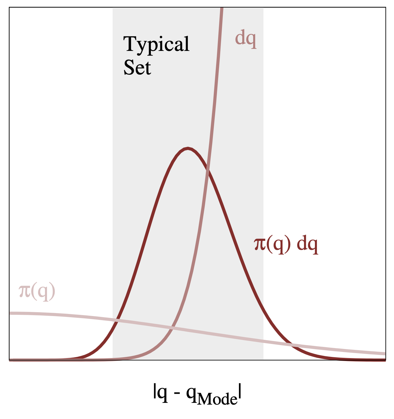
Figure and caption from A Conceptual Introduction to Hamiltonian Monte Carlo, Betancourt, 2017
The typical set is the region where we have both high density and high volume. In high dimensions, it is crucial to think about volume, in that regions with high density don’t necessarily have high volume. In practice, we find the typical set with the sampling process that explores the parameter space.
A popular algorithm is Markov Chain Monte Carlo (MCMC), where we sample from the posterior by exploring the space in an iterative fashion. Each sample define a state in a markov chain, i.e. a sequential discrete process that has no memory, and we explore the space according to some step function.
We can also use Variational Inference, where we approximate the posterior density with a known parameterized family of distributions such as Gaussians that we can optimize with e.g. stochastic gradient descent; in this case, it becomes stochastic variational inference (SVI). Note that the similarity between posterior and the variational distribution is often evaluated with the Kullback-Leibler divergence.
If you need something even more scalable, paying the price of quality, you can use the Laplace approximation 1.
The detailed machinery of inference algorithms are out of scope for this blog post, but the workhorse of modern bayesian inference. Indeed, for many problems the inference using e.g. MCMC is very computationally intensive, so scalable techniques are highly desired.

Back to the repeated coin toss problem
We’re going to solve the coin toss problem with Python and Numpyro, a probabilistic programming library based on JAX. We are going to explore full posterior inference with a MCMC algorithm (in our case the No U-Turn Sampler or NUTS).
Uniform prior
Let’s assume a uniform prior for the bias of the coin, that is any bias is equally likely. Note that you can make one side of a coin heavier, so that it is biased, but I doubt that we could have a coin that always leads heads.
Anyways, as a first step let’s try this model.
First, let’s import the packages we need
import numpy as np
import matplotlib.pyplot as plt
import pandas as pd
import numpyro as ny
import numpyro.distributions as dist
from numpyro.infer import MCMC, NUTS, Predictive
from jax import random

plt.style.use('ggplot')
%config InlineBackend.figure_format = 'svg'
Let’s describe the data. Note that here 1 means heads, so that the observations [1, 1, 1] map to the realizations of our experiments.
tosses = np.asarray([1, 1, 1])
nb_heads = (tosses == 1).sum()
total_tosses = tosses.shape[0]
Then, let us define the model. As discussed above, we use a Uniform prior for the bias of the coin. Then, we use a binomial likelihood. The nb_heads parameter use as obs=nb_heads in the likelihood allows us to tell the model to condition on this observation for the inference. This parameter is optional because for prediction we don’t observe it.
def model(N, nb_heads=None):
    p = ny.sample("p_heads", dist.Uniform())
    ny.sample("nb_heads", dist.Binomial(N, probs=p), obs=nb_heads)
Let’s check a prior predictive simulation, i.e. what we would predict without having seen any data. We simulate 1 toss with 10_000 samples from the prior distribution:
prior_predictive = Predictive(model, num_samples=10_000)
all_prior_samples = prior_predictive(random.PRNGKey(5), N=1)
plt.hist(all_prior_samples["p_heads"], bins=30)
plt.title("(Beta) Prior probability distribution of the bias of the coin p(heads)")
prior_preds = all_prior_samples["nb_heads"]
prior_proba_next_heads = (prior_preds == 1).mean()
plt.hist(prior_preds)
plt.title(
    f"Prior predictive probability of next toss to be Heads is {prior_proba_next_heads:.3f}"
)
Nothing surprising, the prior probability of the next toss being heads is approximately 0.5, since we have a uniform prior i.e. all possible biases are equally likely.
Now let’s run the inference using a Markov Chain Monte Carlo (MCMC) algorithm to infer the posterior distribution of the bias of the coin. We also plot this distribution and its mean.
mcmc = MCMC(NUTS(model), num_warmup=1000, num_samples=10000)
mcmc.run(random.PRNGKey(0), N=total_tosses, nb_heads=nb_heads)
posterior_p_heads_samples = mcmc.get_samples()["p_heads"]
plt.hist(posterior_p_heads_samples, bins=30)
plt.axvline(posterior_p_heads_samples.mean(), linestyle="--", color="red", label="mean")
plt.legend()
plt.title("Posterior distribution of the probability of Heads (bias of the coin)")
mcmc.print_summary()
sample: 100%|██████████| 11000/11000 [00:02<00:00, 5274.72it/s, 3 steps of size 1.05e+00. acc. prob=0.92]
mean std median 5.0% 95.0% n_eff r_hat
p_heads 0.67 0.15 0.68 0.43 0.91 3534.42 1.00
Number of divergences: 0
We obtain predictions directly with the Predictive method. Note that since we simulate one toss, this is a Bernoulli experiment thus the predictive probability is exactly equal to the mean.
predictive = Predictive(model, mcmc.get_samples())
preds = predictive(random.PRNGKey(10), N=1)["nb_heads"]
proba_next_heads = (preds == 1).mean()
plt.hist(preds)
plt.title(
    f"Posterior probability of next toss to lead to heads is approx. {proba_next_heads:.3f}"
)
A more realistic Beta prior
Let’s modify the model with a \mathrm{Beta} prior:
def model(N, nb_heads=None):
    p = ny.sample("p_heads", dist.Beta(3, 3))
    ny.sample("nb_heads", dist.Binomial(N, probs=p), obs=nb_heads)
The prior predictive is almost the same since the prior is centered in 1. However, the posterior distribution is very different:

Same as before, since we only simulate one toss, the probability of the next toss being Heads is the mean of the posterior distribution:

Betting on the outcome
As discovered by Bruno De Finetti, our belief about the world should translate into betting odds. In other words, what are the fair odds that you should accept for a given outcome ? The fair decimal odds for a given event of probability p can be obtained by taking odds = {1 \over p}.
Betting on the next coin toss
In the case of a uniform prior, the probability of the next coin toss leading to Heads is 0.8, hence odds of {5 \over 4} = 1.25.
However, with a \mathrm{Beta} prior, we have a probability of 0.68, hence odds of 1.47. Way higher, for the same set of observations !
So, which is the right odds ? Neither. Because there are many scenarios, that is many possible biases, that could lead to the sequence Heads - Heads - Heads as the first three tosses. As Michael Betancourt would say, embracing uncertainty with probability is what makes us bayesian. Hence, not focusing on the mean of the posterior distribution of p_heads but rather checking the whole extent of the density. This gives us plenty of information, from which we can draw credible intervals if we want.
As Georges Box famously said:
All models are wrong, but some are useful.
We could even argue that the true probability of an event doesn’t exist, it is merely a way to measure our incomplete information about the world in a specific context. In the real world, there is no probability, only events that happen or don’t happen. But what about quantum physics ? Well, we don’t deal with such a small scale here so I argue it’s irrelevant. We got a bit sidetracked, and to be honest this stuff is over my head.
Note: I wrote a bit more about how to translate probabilities to bets if you are interested in this stuff.
Conclusion
If by now you are not at least a little bit Bayesian, you must be deep into the frequentist cult! Joke aside, I hope that the mysteries of bayesian inference are now a bit less obscure, and that you will produce lots of great models with probabilistic programming.
Many thanks to Théo Stoskopf, Théo Dumont, Haixuan Xavier Tao, Ai-Jun Tai for their precious feedback on early drafts of this post
Footnotes
Reuse
Citation
@online{guy2024,
  author = {Guy, Horace},
  title = {An Introduction to Bayesian Inference},
  date = {2024-04-24},
  url = {https://blog.horaceg.xyz/posts/bayes/},
  langid = {en}
}